What can Madden tell us about the NFL?
library(RCurl)
library(ggplot2)
library(dplyr)
library(wordcloud)
The Madden NFL 16 video game was released last Tuesday. To build hype for the release of its new product, EA Sports featured a series of ratings reveals (i.e., ratings of players and teams to be featured in the new game). In addition to new gameplay features, ratings are highly anticipated year after year. EA Sports actually posted a segment in which viewers can watch NFL rookies react to their ratings for the first time.
At the conclusion of its ratings series, EA Sports posted a spreasheet containing all player and team ratings. In addition to overall ratings, it includes skill ratings as well—things like speed, throw power, block shedding, route running, tackling, etc.
I decided that it may be interesting to address some questions concerning the NFL (from Madden’s perspective) using this dataset.
The Data
First things first, I read the Ratings Spreasheet (as two .csv files) into R and cleaned up the dataset.
players = read.csv(text=getURL("https://raw.githubusercontent.com/jskaza/data/master/madden-ratings/Base%20Set%20Players-Table%201.csv"))
teams = read.csv(text=getURL("https://raw.githubusercontent.com/jskaza/data/master/madden-ratings/Teams-Table%201.csv"))
# painless data cleanup
# returns string w/o trailing whitespace
trim.trailing = function (x) sub("\\s+$", "", x)
# remove extra column
players$X = NULL
# remove extra row
players = players[-c(2327), ]
# remove extra whitespace
players$Team = trim.trailing(players$Team)
# remove extra column
teams$X = NULL
# remove extra row
teams = teams[-c(33), ]
# generate mean player rating variable
team_mean_OVR = aggregate(OVR~Team, players, mean)
teams = merge(teams, team_mean_OVR, by.x = 'Nickname', by.y = 'Team')
Once that was taken care of, I was ready to tackle the following questions.
Are the teams with the most talented players the best teams?
This is a question that is adressed in sports all of the time. In basketball, there is the classic case of the 21st century Spurs not necessarily having the most talent in the NBA but being the best team because of the way its players function as one. In other words, ‘the whole is greater than the sum of its parts’.
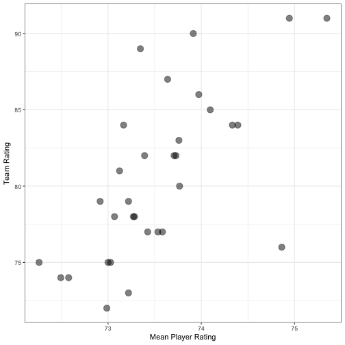
The Madden data presents an interesting way to tackle this question in the context of the NFL. Namely, there are overall team ratings and overall player ratings. I am not sure how the Madden ratings czar determines overall team ratings—and, specifically, whether or not they are a function of the individual player ratings—but if the best teams are the ones with the most talent, there should be a direct relationship between team rating and average player rating. While the plot below suggests that there is a positive correlation between these two metrics, it is not perfect ($r$ = 0.662).
# the base plot
p1 = ggplot(data=teams, aes(OVR,TEAM.OVR)) + geom_point(alpha=.5, size=4) + xlab("Mean Player Rating") + ylab("Team Rating") + theme_bw()
# add linear fit and select labels
p2 = p1 + stat_smooth(method="lm", se=FALSE, size=2) + geom_text(data=subset(teams, Nickname == "Jets" | Nickname == "Patriots" | Nickname == "Seahawks" | Nickname == "Redskins" | Nickname == "Titans" | Nickname == "Packers" | Nickname == "Broncos"), aes(OVR,TEAM.OVR,label=Nickname), hjust=.5, vjust=1, angle=35) + xlim(min(teams$OVR)-.25, max(teams$OVR)+.25) + ylim(min(teams$TEAM.OVR)-2, max(teams$TEAM.OVR)+2)
# display base plot
p1

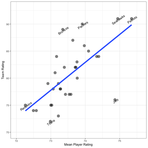
Adding a simple linear fit can add a bit more clarity and can help in identifying the interesting cases.
p2 # display linear fit & labels

We see that the Patriots and Seahawks—both participants in Super Bowl XLIX—have the most talented rosters and are rated as the top two teams in the league. On the other end of the spectrum, for the Redskins and Titans, it appears that a lack of talented players may be a factor in a low team rating.
The other three teams highlighted in the chart represent much more interesting cases. Given the talent level of the average player on their respective rosters, the Packers and Broncos each have team ratings higher than is expected. On the other hand, the Jets have the third highest mean player rating in the league but possess a miserable team rating. My guess is that quarterback play may have something to do with these anomalous cases. Specifically, I think that the quarterback’s rating has a relatively high influence on a team’s rating, seeing that it is well known that QB play can make or break a team. The Packers and Broncos may have decent—but not elite—rosters overall. However, both teams possess stellar quarterbacks. In fact, Green Bay quarterback Aaron Rodgers is one of three players in the entire game to receive the coveted 99 overall rating. On the other hand, it is no secret that the Jets lack talent at the quarterback position.
Who are the most athletic players in the game?
To answer this question, I created a new variable equalling the sum of a player’s speed, strength, and jumping ratings: \(Athleticism = Speed + Strength + Jumping\) Clearly this is a simple metric but I think it captures the basic elements of athleticism. Every category takes on ratings values from 0 to 99, so, for reference, the maximum possible $Athleticism$ score would be 297. Below are the 20 highest rated players.
# create Athleticism metric
players$Athleticism = players$Speed + players$Strength + players$Jumping
players_athletic = players[order(-players$Athleticism),]
# top 20
players_athletic = players_athletic[1:20,]
print(subset(players_athletic, select = c(Team, First.Name, Last.Name, Position, Athleticism)), row.names = FALSE)
##        Team First.Name   Last.Name Position Athleticism
##    Steelers       Ryan     Shazier      MLB         272
##       Bears  Cornelius  Washington     ROLB         269
##       49ers     Vernon       Davis       TE         268
##     Vikings     Adrian    Peterson       HB         268
##     Falcons        Vic Beasley Jr.       RE         267
##       Lions     Calvin     Johnson       WR         265
##    Seahawks  Christine     Michael       HB         265
##    Patriots LeGarrette      Blount       HB         264
##     Raiders     Khalil        Mack     LOLB         264
##     Broncos  Demaryius      Thomas       WR         262
##     Falcons      Julio       Jones       WR         262
##       Lions     Julian    Stanford     ROLB         262
##      Texans       J.J.        Watt       RE         262
##     Vikings     Jerick    McKinnon       HB         262
##      Chiefs      Chris      Conley       WR         261
##     Cowboys        Dez      Bryant       WR         261
##     Cowboys      Byron       Jones       CB         260
##    Seahawks    Richard     Sherman       CB         260
##  Buccaneers    Vincent     Jackson       WR         259
##    Seahawks     Robert      Turbin       HB         259
What is the most prevalent name in the league?
Answering this question just gave me a reason to test out the wordcloud package. The interpretation of the wordcloud is straightforward: larger text means more prevalent name. For what it’s worth, the most popular names in the game (at least at the time of its release) are Chris and Brandon.
pal = brewer.pal(9,"BuGn")
pal = pal[-(1:4)]
name_count = count(players, First.Name)
wordcloud(words=name_count$First.Name, freq=name_count$n, min.freq=3, colors=pal)

How do the QBs stack up?
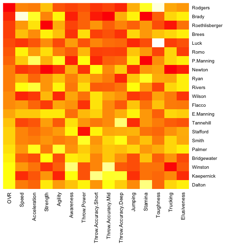
How could one write an article on the NFL without discussing quarterbacks? To satisfy this obligation, I created a graphic that compares all QBs meeting the following condition: \(Overall \, Rating \, (OVR) \ge 80\) This reduces the size of the QB pool to 21 and makes the graph much more readable. The plot orders quarterbacks based on $OVR$ (Aaron Rodgers (99) - Andy Dalton (80)) and includes a number of ratings categories important for quarterbacks. Darker squares indicate relatively high ratings.
It is clear why Rodgers receives the top overall mark. He possesses high ratings accross the board. The class of young and mobile quarterbacks, which includes Colin Kaepernick, Russell Wilson, Cam Newton, and Andrew Luck, is easy to pick out due to those players’ high $Speed$ and $Agility$ scores. The older generation of pocket passers—e.g., Brady, Brees, and Manning—may not have the quickness but boast remarkable $Accuracy$ ratings.
# create heatmap for qb ratings
qb = subset(players, Position=="QB" & OVR >= 80, c(Last.Name, OVR, Speed, Acceleration, Strength, Agility, Awareness, Throw.Power, Throw.Accuracy.Short, Throw.Accuracy.Mid, Throw.Accuracy.Deep, Jumping, Stamina, Toughness, Trucking, Elusiveness))
qb = qb[order(qb$OVR),]
# distinguish b/w manning bros.
qb$name = ifelse(qb$Last.Name != "Manning", as.character(qb$Last.Name), ifelse(qb$OVR == 92, "P.Manning", "E.Manning"))
qb1 = qb[,-1]
qb1$name = NULL
rownames(qb1) = make.names(qb[,ncol(qb)], unique=TRUE)
qb_matrix = data.matrix(qb1)
qb_heatmap = heatmap(qb_matrix, Rowv=NA, Colv=NA, col = rev(heat.colors(256)), scale="column", margins=c(10,10))

