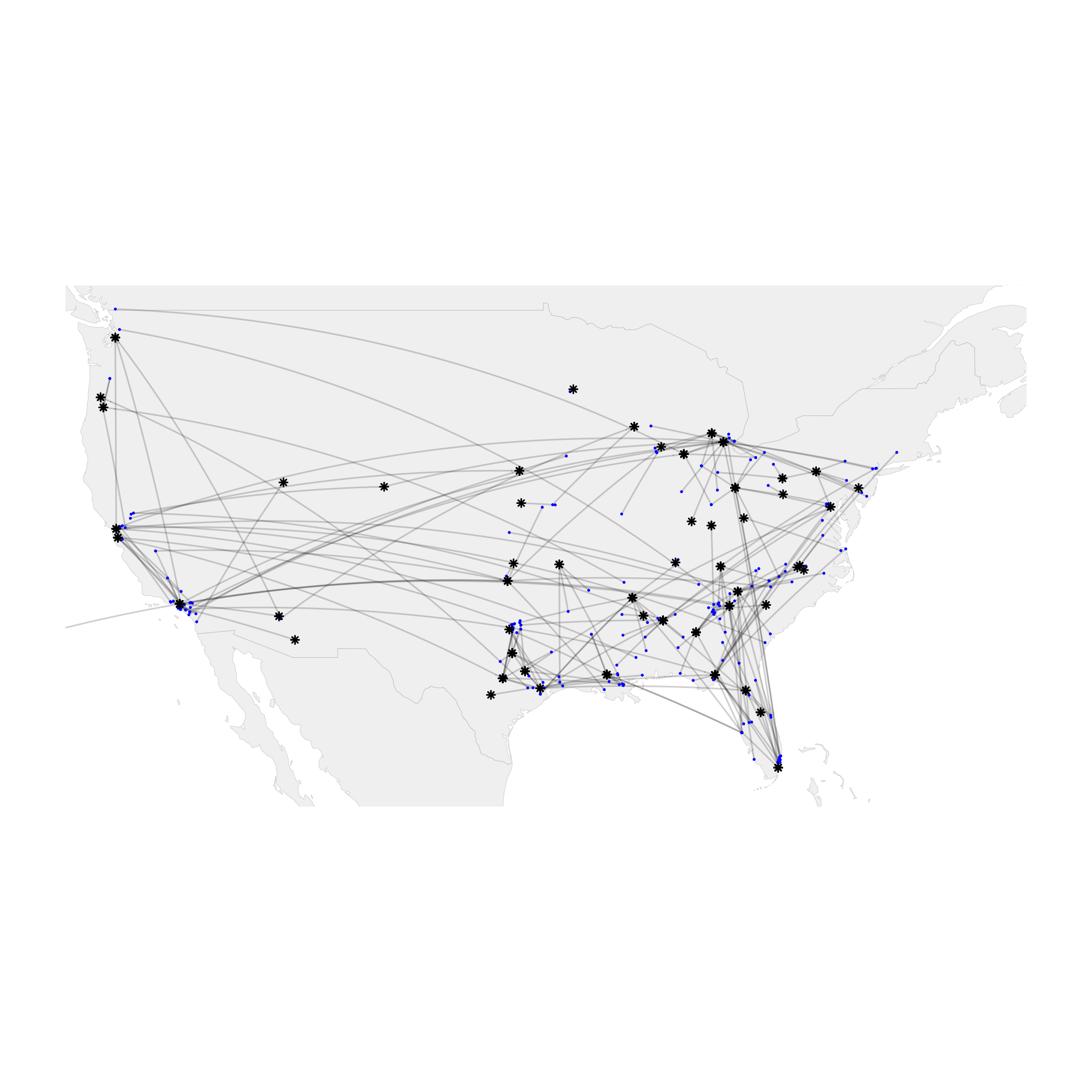
2016 NCAAF Recruiting Geographic Breakdown
With college football less than 100 days away, here is a look at just how far 250 of the nation’s top incoming prospects have to travel to get to their chosen colleges.
The prospect data come courtesy of Rivals, while I obtained school location data from Wikipedia.
The small blue dots represent hometowns and the larger black stars represent colleges and universities.
R Code is included below while my data wrangling code is posted to my GitHub.
library(maps)
library(geosphere)

master = read.csv("../data/recruiting-geography/master.csv")
col = rgb(7, 7, 7, 50, maxColorValue = 255)

xlim <- c(-125, -65)
ylim <- c(24, 50)

map("world", col="#f2f2f2", fill=TRUE, bg="white", lwd=0.05, xlim=xlim, ylim=ylim)
for (i in 1:length(master$X)) {
inter = gcIntermediate(c(master[i,]$home_lng, master[i,]$home_lat),
                       c(master[i,]$school_lng, master[i,]$school_lat), n=100, addStartEnd=TRUE)

lines(inter, col=col, lwd=1)
}

points(master$home_lng, master$home_lat, col='blue', cex=.25, pch=16)
points(master$school_lng, master$school_lat, col='black', cex=.5, pch=8)

