The Best Draft Pick in the Lottery Era
To determine the best draft pick in NBA history, it is first necessary to establish some ground rules, since the NBA Draft is everchanging. To remove some of the inter-draft variation, I will confine the analysis to drafts of the Lottery Era (1985-present). Additionally, I will only consider selections made with picks 1-60 in each draft, as the NBA Draft included more than two rounds in the late 1980s. The NBA Draft has featured exactly 60 selections each year since 2005.
My definition of the best draft pick is the player who performed best throughout his career relative to expectations. I am not concerned with whether a player was traded or left a team—just where he was drafted and how he performed over the course of his career. There are three important components to my defintion, each of which is worth elaborating upon.
-
“the player who performed best”. There are many ways to assess performance in basketball—points, rebounds, assists, +/-, efficiency—the list goes on and on. However, in this analysis I will use Win Shares (WS), an estimate of the number of wins directly attributable to a player.
-
“throughout his career”. A truly successful draft pick does not provide value to his team(s) for a season or two, but instead enjoys a sustained run of good play for many years. In this regard, it is difficult to deem a rookie or second year player a great draft pick because of the small sample size.
-
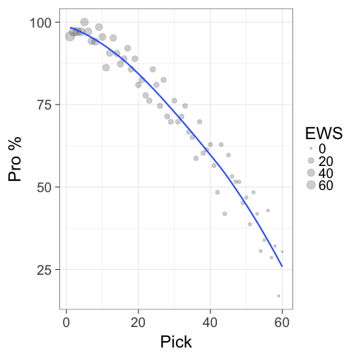
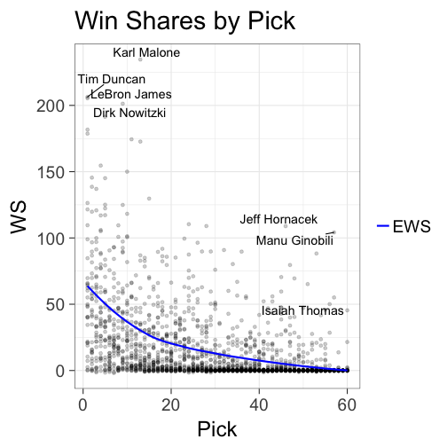
“relative to expectations.” To fairly evaluate a draft pick, one must be mindful of where that player was selected. The player picked first in the draft is expected to have a better career than the player picked 20th in the draft. In fact, there is a decent chance that a player picked late in the draft will never actually make it to the NBA. Basketball Reference has expected career WS (EWS) for each pick in the draft. The first pick is expected to produce 76.9 WS over the course of his career, compared to 20.6 for the 20th selection. A good draft pick will outdo his expected level of production, as well as the levels of production of other players picked in the same slot.
library(readxl)
library(ggplot2)
library(XML)
library(RCurl)
library(rlist)
library(tidyverse)
library(ggrepel)
library(knitr)
# EWS data
EWS = read.csv(text=getURL("https://raw.githubusercontent.com/jskaza/data/master/nbadraft2017/draft_data.csv"))
EWS$Pro. = as.numeric(gsub("\\%", "", EWS$Pro.))
ggplot(data=EWS, aes(x=Pk, y=`Pro.`, size=EWS)) + geom_point(alpha=0.2) +
  geom_smooth(se=FALSE, show_guide=FALSE) + xlab("Pick") + ylab("Pro %") +
  theme_bw(base_size = 24)
## Not Run ##
## Used to scrape data ##
# obtain data for picks 1-60 since 1985
theurl = getURL("http://www.basketball-reference.com/play-index/draft_finder.cgi?request=1&year_min=1985&college_id=0&pick_overall_min=1&pick_overall_max=1&pos_is_g=Y&pos_is_gf=Y&pos_is_f=Y&pos_is_fg=Y&pos_is_fc=Y&pos_is_c=Y&pos_is_cf=Y&order_by=year_id",.opts
= list(ssl.verifypeer = FALSE))
tables = readHTMLTable(theurl)
tables = list.clean(tables, fun = is.null, recursive = FALSE)
n.rows = unlist(lapply(tables, function(t) dim(t)[1]))
picks = as.data.frame(tables[[which.max(n.rows)]])
for (pick in 2:60){
  theurl = getURL(paste0("http://www.basketball-reference.com/play-index/draft_finder.cgi?request=1&year_min=1985&college_id=0&pick_overall_min=",as.character(pick),"&pick_overall_max=",as.character(pick),"&pos_is_g=Y&pos_is_gf=Y&pos_is_f=Y&pos_is_fg=Y&pos_is_fc=Y&pos_is_c=Y&pos_is_cf=Y&order_by=year_id"),.opts = list(ssl.verifypeer = FALSE))
  tables = readHTMLTable(theurl)
  tables = list.clean(tables, fun = is.null, recursive = FALSE)
  n.rows = unlist(lapply(tables, function(t) dim(t)[1]))
  new_picks = as.data.frame(tables[[which.max(n.rows)]])
  picks = rbind(picks, new_picks) }

# remove extra rows
picks = picks[!(picks$Rk=="Rk" | picks$Lg=="Per Game"),]

# convert Pick # and WS to numeric
picks$Pk = as.numeric(as.character(picks$Pk))
picks$WS = as.numeric(as.character(picks$WS))

# blank WS -> 0 WS
picks[c("WS")][is.na(picks[c("WS")])] = 0
# load scraped data
picks = read.csv(text=getURL("https://raw.githubusercontent.com/jskaza/data/master/nbadraft2017/picks.csv"))

# plot WS vs. pick and add EWS line
EWS$WS = EWS$EWS
ggplot(data=picks, aes(x=Pk, y=WS)) + geom_point(alpha=0.2) +
  geom_smooth(data=EWS, se=FALSE, aes(col="EWS")) +
  # add labels for interesting cases
  geom_text_repel(data=subset(picks, WS > 200| (WS > 100 & Pk > 40) |
                                (WS > 40 & Pk == 60)),
            aes(Pk,WS,label=Player), size=5) + xlab("Pick") +
  ggtitle("Win Shares by Pick") + scale_colour_manual(name="",values=c("blue")) +
  theme_bw(base_size = 24)
There are numerous ways to measure how much a player $i$, selected with pick $j$, exceeds his EWS. However, I will focus on two such metrics.
- $WSEWS_{ij} = WS_i/EWS_j$
- $Z_{ij} = (WS_{ij} - EWS_j)/SD(WS_j)$
The first metric is rather straightforward. We evaluate a player’s performance simply as a ratio of his WS to his EWS. $WS/EWS$ > 1 indicates good performance relative to expected performance.
Interestingly, the EWS for the 60th pick is actually -0.1 (the only pick with $EWS < 0$). This indicates that the 60th pick is actually expected to make a negative contribution over the course of his career. However, a negative EWS will invalidate the WSEWS statistic, seeing that a player drafted 60th with positive WS will possess a negative WSEWS. To combat this issue, I will replace the EWS for pick 60 with that for pick 59 when computing WSEWS. Because EWS is a monotonically decreasing function of pick number, this is a conservative remedy. In other words, 60th picks are being treated as though they were selected 59th.
# avoid duplicate WS
EWS$WS = NULL
# combine WS and EWS data
combined_data = merge(picks, EWS, by="Pk")
# replace 60th pick EWS with that of 59th pick
combined_data$EWS_revised = ifelse(combined_data$Pk == 60, 0.2, combined_data$EWS)
# WSEWS metric
combined_data$WSEWS = combined_data$WS/combined_data$EWS_revised
# sort by WSEWS and display
ordered_WSEWS = combined_data[order(-combined_data$WSEWS),]
kable(head(ordered_WSEWS, n=10)[,c("Player","Pk","WSEWS")], caption = 'Top 10 Players by WS/EWS', row.names = FALSE, digits=1)
| Player | Pk | WSEWS |
|---|---|---|
| Isaiah Thomas | 60 | 227.0 |
| Manu Ginobili | 57 | 115.8 |
| Drazen Petrovic | 60 | 107.5 |
| Marcin Gortat | 57 | 61.2 |
| Amir Johnson | 56 | 41.8 |
| Anthony Mason | 53 | 38.4 |
| Luis Scola | 55 | 28.6 |
| Ramon Sessions | 56 | 23.8 |
| Don Reid | 58 | 22.8 |
| Jeff Hornacek | 46 | 22.2 |
# plot WSEWS by pick
ggplot(data=ordered_WSEWS, aes(x=Pk, y=WSEWS)) + geom_point(alpha=0.2) +
  geom_text_repel(data=subset(ordered_WSEWS, WSEWS > 50),
                  aes(Pk,WSEWS,label=Player), size=5) +
  xlab("Pick") + ggtitle("WSEWS for Each Pick") + theme_bw(base_size = 24)
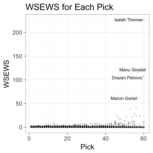
Despite having been “Mr. Irrelevant”—the last selection in the NBA Draft—and only entering his 8th season, the Boston Celtics’ Isaiah Thomas leads all players in WSEWS. It is not surprising that the top list features many very late picks. EWS decreases exponentially with pick number; any late round pick that can accumulate significant WS will possess a very high WSEWS.
The second metric is essentially a z-score, indicating how many standard deviations away a player is from his EWS. For example, a player with $Z=2$ performed 2 standard deviations above expectation.
# function to get Z
normalize = function(x,y){
  return((x-y)/sd(x))
}
# create Z dataset
z_data =
  combined_data %>%
  group_by(Pk) %>%
  mutate(Z = normalize(WS,EWS))
# sort by Z and display
ordered_z = z_data[order(-z_data$Z),]
kable(head(ordered_z, n=10)[,c("Player","Pk","Z")], caption="Top 10 Players by Z", row.names = FALSE, digits=1)
| Player | Pk | Z |
|---|---|---|
| Anthony Mason | 53 | 5.4 |
| Kyle Korver | 51 | 5.3 |
| Jeff Hornacek | 46 | 5.2 |
| Rashard Lewis | 32 | 4.9 |
| Steve Kerr | 50 | 4.7 |
| Clifford Robinson | 36 | 4.7 |
| Don Reid | 58 | 4.5 |
| Manu Ginobili | 57 | 4.5 |
| Marc Gasol | 48 | 4.5 |
| Sam Mitchell | 54 | 4.5 |
# plot Z by pick
ggplot(data=z_data, aes(x=Pk, y=Z)) + geom_point(alpha=0.2) +
  geom_text_repel(data=subset(z_data, (Z > 4.5) | (Z > 3.7 & Pk < 30)), aes(Pk,Z,label=Player), size=4) +
  xlab("Pick") + ggtitle("Z for Each Pick") +
  theme_bw(base_size = 24)
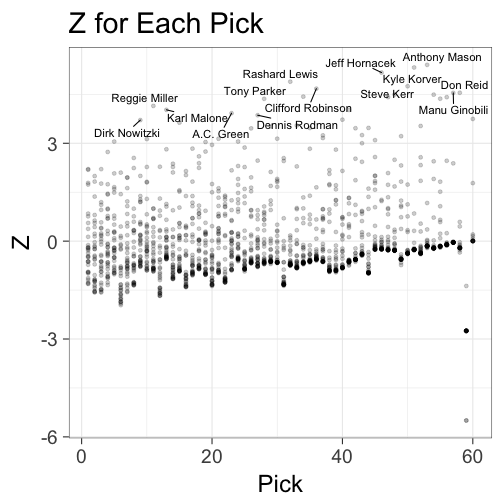
Anthony Mason was selected with the 53rd pick in the 1988 NBA Draft yet produced the second most WS from that draft class. He leads all players in the Z metric. The z-scores are clustered around zero, as is to be expected. On average, a draft pick will produce at his expected level. When compared to WSEWS, the Z metric seems to give more credit to top selections who vastly outperform expectations.
While I like both metrics, they unfortunately produce different rankings and lend different answers to the question of who is the best draft pick. As a compromise, I will create a composite ranking—the average rank in each list.
# create ranks
ordered_WSEWS$rank_WSEWS = seq(1,nrow(ordered_WSEWS))
ordered_z$rank_Z = seq(1,nrow(ordered_z))
# names as characters
ordered_WSEWS$Player = as.character(ordered_WSEWS$Player)
ordered_z$Player = as.character(ordered_z$Player)
# sort by name
z_player = ordered_z[order(ordered_z$Player),]
WSEWS_player = ordered_WSEWS[order(ordered_WSEWS$Player),]
# get avg rank
overall = WSEWS_player
overall$rank_z = z_player$rank_Z
overall$`Avg Rank` = (overall$rank_WSEWS + overall$rank_z)/2
overall_rank = overall[order(overall$`Avg Rank`),]
kable(head(overall_rank, n=10)[,c("Player","Pk","Avg Rank","WS")], caption="Top 10 Players by Average Rank", row.names = FALSE)
| Player | Pk | Avg Rank | WS |
|---|---|---|---|
| Anthony Mason | 53 | 3.5 | 88.3 |
| Manu Ginobili | 57 | 5.0 | 104.2 |
| Jeff Hornacek | 46 | 6.5 | 108.9 |
| Kyle Korver | 51 | 7.0 | 65.2 |
| Don Reid | 58 | 8.0 | 13.7 |
| Amir Johnson | 56 | 9.0 | 50.1 |
| Steve Kerr | 50 | 10.0 | 47.2 |
| Luis Scola | 55 | 10.5 | 45.7 |
| Sam Mitchell | 54 | 10.5 | 41.7 |
| Isaiah Thomas | 60 | 11.0 | 45.4 |
When combining the rankings from both metrics, Anthony Mason emerges as the best draft pick of all-time. A natural question to ask is how can Mason be a better draft pick than Manu Ginobili if Mason was drafted earlier and produced fewer WS? This occurs because there is greater variance in the 57th pick as compared to the 53rd pick. To illustrate, Marcin Gortat, who was also selected 57th, has 55.1 career WS. Hence, by the Z metric, Manu Ginobili’s 104.2 WS is not that anomalous.
The Z metric is largely influenced by the variance in WS for a given pick. By comparison, WSEWS is particularly sensitive to the assumed EWS for a given pick. Another option would be to look at the difference between WS and EWS (by this metric, Karl Malone is far and away the best draft pick of all-time). The reason I am not overly fond of this approach is because it is top-pick heavy. Many of the greatest players of all-time—and hence players with very high WS—were selected early in the draft. I am hesitant to deem someone like LeBron James as one of the greatest draft picks ever because it was a no-brainer for Cleveland to select him. Therefore, without a perfect metric, I will for now claim that Anthony Mason is the best draft pick ever because he vastly outperformed the expectations for a 53rd pick (WSEWS = 38.4) and vastly outperformed other 53rd picks (Z = 5.4).
